Creating Demos - Coder Tutorial #6
[Magnifying Lenses]
By Polaris
A festive greetings to all you demo coders our there! In my home town spring
is finally starting to arrive ... and the relentless winter chill is easing up.
Finally the temperature is rising above -20'c for the first time since November.
This "thaw" reminds me that summer is around the corner. Finally we can start
looking forward to the summer demo parties of 2005!
During the last issue I asked you to vote for the content of the next tutorial.
I got some great correspondence from a student in Portugal.
He's having a blast playing and learning Allegro, and appreciates the focus on
"free tools and compilers". Free tools really fit his tight student budget.
He's requested a tutorial on magnifying lenses, so I'm happy to put the other
tutorial series temporarily on hold to explore how to create a magnifying lens effect.
I'll be using a fair bit of mathematics during this tutorial.
You'll need to understand basic trigonometry (sin, cos, tan), inverse trigonometry
functions, as well as "distance" (Pythagorean Theorem), and have a good comfort for
the Cartesian coordinate system. A good refresher on the web for these concepts
is located in the "Trigonometry: A Crash Review" website. Check it out here:
http://www.zaimoni.com/Trig.htm
I realize this tutorial "jumps right" into some things... but take your time with it.
It might not be entirely understood overnight – but with some effort it should be clear.
As always if you have any specific questions – I'm just an email away.
Lens Physics 101 – What is a lens?
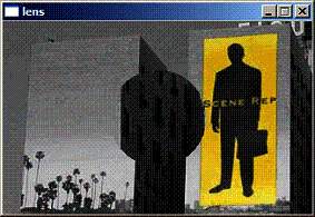
 The first thing we need to do to code a lens effect is to get a basic understanding
of what lenses are and how they work. The effect we are trying to reproduce
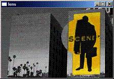
is convex lens; just like a standard magnifying glass. You can see the effect
in the screen capture. The word "scene" is magnified by the virtual lens.
This tutorial will teach you how to make that lens.
The first thing we need to do to code a lens effect is to get a basic understanding
of what lenses are and how they work. The effect we are trying to reproduce
is convex lens; just like a standard magnifying glass. You can see the effect
in the screen capture. The word "scene" is magnified by the virtual lens.
This tutorial will teach you how to make that lens.
I need to stress something very important. We are not attempting to fully model physical
reality – only a perception of it. Our simulation does not need to be physically
accurate. It needs only to "look right". There are many ways to simulate a lens,
and I'm sure that the one that I describe here isn't orthodox. I developed it from
the ground up and it's far simpler to understand and describe than a number of other
lens tutorials. It's also reasonably flexible. The most important piece of the article
isn't so much "the lens" but the speed optimizations we make at the end of the tutorial
to speed up the effect.
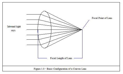
The basic magnifying effect is caused by light refracting with a lens. Light rays get
refracted (bent) by the lens and converge on a single point. This point is also
known as the "focal point" of the lens. Whenever someone ignites something (like paper)
with a magnifying lens – they are taking advantage of the focal point. All the light rays
that intersect with the lens converge and heat up the small focal point to the point
of burning.
Each lens has a different focal point, which results in different powers of magnification.
Many lens systems call this the "Magnification factor" as altering it changes the degree
of magnification. The distance between the lens focal point and the lens is known
as the focal length. This is summarized in figure 1.0.
So far, all these definitions have focused on light traveling towards the focal point.
When a magnifying glass is used - the object for magnification is placed between the
lens and the focal point. Light travels from the object to the lens and then into
the eye. To generate a simple lens effect however, we can imagine the light traveling
in the same fashion as we've already described.
Figure 1.0 shows a "side view", with the Z axis (left to right) and
the Y axis (up and down). This is actually all we really need know to do this effect.
If you hold a lens in front of you – looking towards the Z axis – rotations
along the Z axis don't affect the image. [In other words there is no way to hold
a lens "upside down"]. If we are able to solve equations for our side image - in terms
of Height and Depth (Y and Z) - we have also solved for X because we can treat X the
same exact way.
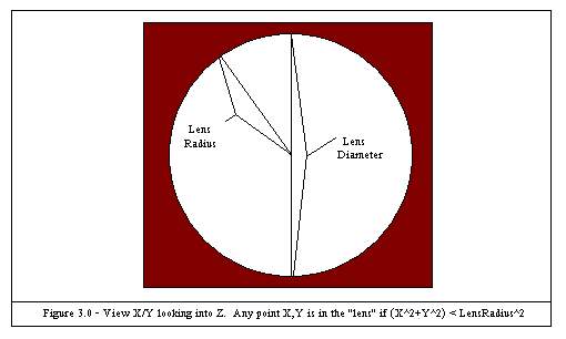
For our simulation there are a few constants we will consider as known. Let us call
the distance from the bottom of the lens to the top of the lens the "lens diameter"
(see Figure 3.0). When we apply the effect onto the computer screen – we'll consider
the lens to be applied to the square occupying the area of Lens_Diameter x Lens_Diameter
(in pixels). We'll simply drop out any points outside of the "lens", but are still in
the area of square [Lens_Diameter x Lens_Diameter]. (Shown in red).
We also know the focal length of the lens, and for simplicity can consider the
focal point to be at the origin of the coordinate system. Similarly, the distance
between the object placement and the focal length is a constant of our simulation – known
as "object_d" – object distance.
We render our lens by looping across the lens surface (diameter), in two loops.
This appears in the following pseudo code.
Lens_radius = ˝ lens diameter
for y=-lens_radius to lens_radius
{
for x=-lens_radius to lens_radius
{
// find out where the light ray intersects the object .
// Set this to p_x and p_y
new_colour=bitmap_get_pixel(p_x,p_y);
bitmap_set_colour(x,y,new_colour);
}
}
Now the pseudo code is a bit naive (for example it doesn't take into account screen
coordinates), vrs "lens coordinates". However from that pseudo code... you can see
that the only thing we really need to know is what the projected X and projected Y are
for a given X,Y. Once we know that - We've solved the magnification equation.
Lens Physics 102 – Solving the Lens Equation
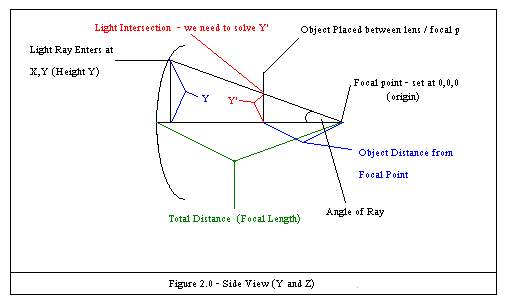
Figure 2.0 shows what we need to solve. We know the focal length of the lens,
and the distance of the object between the lens and the focal point.
We also know Y – the height of the light ray as it enters the lens.
What we need to solve is Y'. Y' is the height of refracted light ray where
the light intersects our magnified object.
I've seen lots of tutorials that show how to solve this, and only a few use trigonometry.
Most rely heavily on the Pythagorean theorem. I realize that some people might avoid
trigonometry based on its computation speed.. and that's rightly so. However – it's
possible to almost completely pre-calculate the lens with optimization.
In my opinion – a bit of trigonometry at the initialization phase of the program
isn't anything to be worried about.
When examining Figure 2.0 you might notice that the triangle formed by
the line segment Y (with the other two line segments going to origin) is similar
to the triangle formed by Y' (and the other two line segments going to origin).
In fact – the angle "angle of ray" is shared by these two triangles.
If we know the angle, Y' can be calculated as follows.
TAN(Angle) =(Y' / Object Distance). Y' = TAN(Angle) * Object Distance.
Still, we need to find out the angle in order calculate Y'. You might notice
that the focal length of the lens – is also the length of the line segment from
the light ray entering the lens to the focal point.
We also know the value of Y.
From these two we know that SIN(angle)=(Y/Focal Length).
Taking the inverse sign – we can solve for the angle = asin(y/focal_length).
(Remember asin is simply the inverse sin).
Wow! At this point we can know that Y'=tan(asin(Y/R))*object_d, and can
compute Y' in a program.
Part #1 – Rendering The Lens – 6 Steps to Lens!
Anyone that has been following the tutorials will have a lot of familiarity
in setting Allegro up and making a basic framework. If you don't, go back
to previous chapter and read! Since this is review for most people,
I've created a "basic" framework to start with. Take lens.a.rar from the bonus pack,
and open it up. You'll notice it also includes a pcx image we'll use in this part
of the of the tutorial. The only thing that's a little different with this
framework from code we've already used – is that it initializes the mouse
(as we'll be using the mouse later on).
Now that we've got the framework installed – we need to start coding our effect.
Here is a step by step guide.
1. To start – we'll add some global variables under the namespace. Add:
"BITMAP *bkg_bmp; // the image from the pcx file
PALETTE bkg_pal; // the palette from the pcx file
2. Next up – we'll add our function to draw the lens. I'll go over the function
in detail – but for now... place this into the code. It should already be making
some sense to you.
void draw_simple_lens(float lens_diameter,float focal_length,
     float object_d,int lens_x,int lens_y)
{
    int lens_radius;
    int x,y;
    int p_x,p_y; // projected x, projected y
    int p_c;

    lens_radius=(int)lens_diameter/2;

    for (y=-lens_radius;y<lens_radius;y++)
    {
        for (x=-lens_radius;x<lens_radius;x++)
        {
                if (x*x + y*y<lens_radius*lens_radius)
                {
                // yeah! we are in the "lens circle"
                p_y=tan(asin(y/focal_length))*object_d;
                p_x=tan(asin(x/focal_length))*object_d;

                p_c=_getpixel(  bkg_bmp,
                                p_x+lens_x+lens_radius,
                                -p_y+lens_y+lens_radius);

                _putpixel(screen,
                                x+lens_radius+lens_x,
                                -y+lens_radius+lens_y,
                                p_c);

                }

        }
    }
}
3. In our main program main() – we'll add some constants – that we'll use later on.
These define our lens diameter, lens focal distance, and placement of the object
in the lens:
    // main constants
    const float lens_diam=100;  // constants for lens
    const float lens_focal=80;
    const float lens_place=40;
4. At the point of // init more stuff (next phase) – we need to load our background,
and set the palette. We'll also apply the effect to the screen [once]. Because we
aren't doing any double buffering yet – the effect would "flicker" too badly for us
to see it if we updated in the render loop.
    // init more stuff  (next phase)
    bkg_bmp = load_bitmap("backgrnd.pcx", bkg_pal);  // image load
    set_palette(bkg_pal);      // use image palette

    blit(bkg_bmp, screen, 0, 0, 0, 0, screen_x, screen_y);
    draw_simple_lens(lens_diam,lens_focal,lens_place,110,50);

      // The last line – draws a simple lens at 110,50 of the screen.
5. Remove the "text out" in the "// DO SOMETHING AMAZING HERE!" area
textout(screen, font, "Do Something amazing here!", 0, 0, 255);
6. We've allocated a bitmap to hold the background. We also need to de-allocate it.
// de-init more stuff  (next phase)
destroy_bitmap(bkg_bmp);     // release bitmap data
 That's all there is to it! Give it a compile... and you'll see the lens get drawn
on the screen. You might even add a rest(1) underneath the put pixel – so you can
see the lens get drawn "bottom up" and from left to right. [Note that this will
really slow the drawing down, but will "show you" how it's drawing. Like Slow Motion :-)]
That's all there is to it! Give it a compile... and you'll see the lens get drawn
on the screen. You might even add a rest(1) underneath the put pixel – so you can
see the lens get drawn "bottom up" and from left to right. [Note that this will
really slow the drawing down, but will "show you" how it's drawing. Like Slow Motion :-)]
If everything worked correctly – you should be able to run the application and
enjoy your lens effect as the screen shot shows.
Draw Simple Lens Procedure – In Detail
Over all the simple lens procedure should make sense, however there are a few things
that I haven't yet explained that might be a bit confusing. Let's start with the basics.
The first thing we do is calculate the radius of the lens. We can easily do this,
by finding one half of the lens diameter. You can also see this in Figure 3.0.
Then we loop against the radius of the lens. Notice – we are using the proper
Cartesian coordinate system here.
(These are Cartesian coordinates, not screen coordinates). As such:
- upper left coordinate of the lens == <-R,R>
- upper right coordinate of the lens == <R,R>
- lower left coordinate of the lens == <-R,-R>
- lower right coordinate of lens == <R,-R>
So, we loop against the lens surface in X and Y. Inside the inner loop
we have to determine if the point X,Y is actually inside our lens.
Points outside the lens are in coloured in red in Figure 3.0, and are dropped out
of the equation. This is the only spot of our system where we make use of
the Pythagorean theorem.
Consult figure 4.0 to better understand this. Remember – our coordinate system
is centered with the lens center being <x = 0, y = 0>. Our circle has a radius
of one half the diameter. If point X,Y in question is further from the center than
the length of circle radius – it's outside the circle.
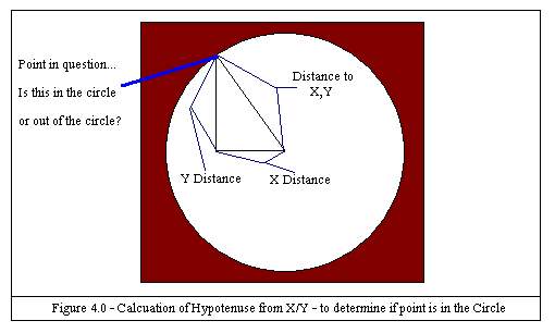
The Pythagorean theorem states that the hypotenuse squared is equal to the sum of
the other two segments squared (for a right triangle). This means that
(Distance to X,Y)^2 = (Y Distance)^2+(X Distance)^2. (Where ^2 means "squared".)
We can calculate the distance to X,Y by taking the square root(x^2, y^2).
A point is in the circle if square root(x^2, y^2) < radius.
Now you might be confused by the code. We aren't using square root, instead it is:
"if (x*x + y*y<lens_radius*lens_radius)". This is strictly a speed optimization.
Since square roots are expensive, we simply square either side of the relationship.
We loose the square root, and compare it against the square of the radius.
At this point we can calculate our projected X and projected Y, with our following
two functions:
1. p_y=tan(asin(y/focal_length))*object_d;
2. p_x=tan(asin(x/focal_length))*object_d;
This is simply an application of the formula we derived in "Lens Physics 102 – Solving
the Lens Equation", Y'=tan(asin(Y/R))*object_d. P_x and P_y are still in pure
Cartesian coordinates.
Now that we have calculated "where" the projected X and Y land – we need to look up
the colour in the background bitmap. Here is where we have to convert to screen
coordinates. Let's compare with our lens coordinate system to screen coordinates.
Remember: Our lens starts at Lens_X, Lens_Y (at upper left, not the middle of the lens).
We feed Lens_X and Lens_Y into our calculations to allow us to move the lens
on the screen.
- upper left coordinate of the lens
== <-R,R>       ==       <Lens_X, Lens_Y>

- upper right coordinate of the lens
== <R,R>        ==        <Lens_X+Lens_Diameter, Lens_Y>

- lower left coordinate of the lens
== <-R,-R>     ==        <Lens_X+Lens_Y+Lens_Diameter>

- lower right coordinate of lens
== <R,-R>       ==        <Lens_X+Lens_Diameter,Lens_Y+Lens_Diameter>

* Where R is the lens radius
Our Y loop starts at the bottom of the lens, and moves to the top.
Y gradually moves from being negative at the bottom of the lens – to growing positive
at the top of the lens. This is proper for the pure Cartesian system – but it's reverse
from how we do screen coordinates. In screen coordinates – the bottom is larger than
the top. We have to compensate for this when we convert Cartesian coordinates to screen
coordinates. We do this by flipping our Y value (taking the negative) – and adding the
lens radius. Adding the lens radius offsets the Y value so it isn't negative.
ScreenY= -lens_ Cartesian _y+lens_radius (note: formula is not yet complete)
ScreenY now starts as a large number, and continues to shrink as we move up the loop.
When it hits 0 – we are at the top of the lens. Since our lens starts at Lens_Y – we offset
this for our final formula (allowing us to move the lens):
Formula A. ScreenY= -lens_ cartesian_y+lens_radius+lens_y. (complete formula).
The x calculation is a little more straightforward. Screen X grows from left to right,
just like the Cartesian coordinate system. All we need to do is "offset it" by the radius
to get only positive values. Adding lens_X also takes into account the starting position
of the lens. Our final ScreenX formula become:
Formula B. ScreenX= lens_ cartesian _x+lens_radius+lens_x;
At this point the rest of the code should make complete sense. We look up the pixel
at p_x and p_y, by using _getpixel against the background image we are magnifying.
You can see the application of Formula A and Formula B – to pass in true screen
coordinates.
The same formulas are used to put the pixel on screen. Voila! There is still much to do
for a really cool lens effect. Let's keep coding!
Part #2 – Animating the Lens
In order to animate the lens following the mouse, we'll have to poll the mouse, and use
double buffering [or it will flicker badly]. Let's add these features step by step.
1. Add the off screen buffer with the other global bitmap declarations.
BITMAP *off_screen; // off screen buffer
2. Rename draw_simple_lens to draw_lens (so we don't confuse it with the other version).
3. Alter the putpixel in draw_lens to go to off_screen instead of screen.
(Rendering to the double buffer).
_putpixel(off_screen,
          x+lens_radius+lens_x,
          -y+lens_radius+lens_y,
          p_c);
4. In the init phase we'll need to create the double buffer and delete it.
In addition we'll want to restrict the mouse movement so we can move the lens
outside the boundary of what's possible. Our init phase ends up looking like this
(notice the removal of the call to blit / draw lens – we'll add those into the
main render loop).
// init more stuff  (next phase)
bkg_bmp = load_bitmap("backgrnd.pcx", bkg_pal);  // image load
set_palette(bkg_pal);      // use image palette
set_mouse_range(0, 0, screen_x-lens_diam-1, screen_y-lens_diam-1);
off_screen = create_bitmap(screen_x, screen_y);

// main loop (see step 5)

// de-init more stuff  (next phase)
destroy_bitmap(bkg_bmp);        // release bitmap data
destroy_bitmap(off_screen);
5. In the main loop – we'll blit the background to the double buffer,
apply the lens, and then blit it to the screen. We'll also use the mouse
instead of static x/y position.
// DO SOMETHING AMAZING HERE!
blit(bkg_bmp, off_screen, 0, 0, 0, 0, screen_x, screen_y);
poll_mouse();
draw_lens(lens_diam,lens_focal,lens_place,mouse_x,mouse_y);
vsync();
blit(off_screen, screen, 0, 0, 0, 0, screen_x, screen_y);
Voila! We've now added double buffering, and can interactively move the lens around!
However – there's plenty more tricks where that came from. Right now our routine is
terribly slow. We've got tangents, multiplies, inverse sins... for every single pixel
of the lens. There has to be a better way and there is!
Part #3 – Moving the Lens to Warp Speed
If you look at the loop – you might notice that our calculations for p_x and p_y don't
actually ever involve lens_x and lens_y. That code is all the same, right up to the point
where we move them into screen coordinates. In fact every iteration of the
loop – p_x and p_y are the same each frame, each time.
The lens affects the projection the same way no matter where it's at. If it moves a pixel
"right" 10 units (from the starting point of the lens), it will do that every single time.
This means that we can pre-calculate the lens in an array of transformations – and then
apply these transformations when we are running. Doing this saves all the overhead of the
somewhat expensive trigonometric functions.
For every point of the lens [x,y] – we can figure out how the light is refracted, and
store the delta of that value into an array. Then we can simply look up how the lens
refracts point X,Y, grab the colour and plot! We don't even need to think about "pure"
coordinate systems versus screen coordinates.
For example – let's say that X becomes X+5 but that Y stays the same. We can represent
that transformation as 5. If x moved 5 points to the left after the transformation – we
could represent that as -5. It's like a pirate counting "paces" on a map.
Y values can be represented the same way. Imagine if we transformed the point
"320 pixels to the right". Well, that falls out of boundary of the 320x200 Mode 13h
screen! What if instead of falling out of bounds – we simply wrapped around..
to the start of the next line. Since each line is 320 pixels – a transformation
of 320 would result in dropping down to Y+1.
Screen coordinates actually use this already. Imagine for a moment if we numbered
all the pixels in a 320x200 grid. Starting at 0 at the top left, we'd count pixels
from left to right to form the first line of the screen – stopping at the right boundary
with pixel 319. If we continued on the next line – we'd encounter pixel 320, and could
continue till we hit the edge at 639. In essence – we can linearly enumerate all
the pixels in the 320x200 video mode – by assigning an ever increasing number depending
on pixel position. (See the table below).
If we wanted to find out what linear position a given X and Y on screen are at – we'd
calculate linear position = y * 320 (number of pixels per screen row) + x.
In this manner if we wanted to represent the transformation of a point Y where Y increases
by 5 units (i.e. goes down 5 units) (but X stays the same) – the transformation would be
equal to 320*5 or 1600. It's possible for us to represent how a point changes both in X
and Y based on one number alone.
Video memory [and the bitmaps] are actually represented in this way. (Mode13 bitmaps
in allegro anyway). This is not always the case in all video modes, but lucky for us
it is for Mode 13h. This means we can really start to optimize our lens effect.
Let's get started!
1. Add an array to hold our transformations - and define a maximum lens size
(at the top of the program – under #define screen_y add):
#define max_lens_diameter 256
int lens_offsets[max_lens_diameter*max_lens_diameter]; // total lens offsets
2. We need to now create this "lens_offsets" table.
This is actually tightly based on the first lens drawing code.
Add this code into your project.
void create_lens(float lens_diameter,float focal_length, float object_d)
{
    int lens_radius;
    int x,y;
    int p_x,p_y; // projected x, projected y

    int p_c;
    int i;

    lens_radius=(int)lens_diameter/2;

    if (lens_diameter>=max_lens_diameter)
    {
        set_gfx_mode(GFX_TEXT, 0, 0, 0, 0);
          allegro_message("Create lens call exceeded max lens.");
          exit(-1); // force abort
    }

    i=0;
    for (y=-lens_radius;y<lens_radius;y++)
    {
        for (x=-lens_radius;x<lens_radius;x++)
        {
                if (x*x + y*y<lens_radius*lens_radius)
                {
                  // yeah! we are in the "lens circle"
                  p_y=tan(asin(y/focal_length))*object_d;
                  p_x=tan(asin(x/focal_length))*object_d;

                  // now - translate p_y, p_x to screen co-ordinates
                  p_x=p_x+lens_radius;
                  p_y=-p_y+lens_radius;
                }
                else
                {
                  p_x=x+lens_radius; // no transformation - screen co-ordinates
                  p_y=-y+lens_radius;
                }

                // gets linear offset.
                lens_offsets[i]=p_y*screen_x+p_x;

                i++;
        }
    }
}
We also need a function that draws the lens using the transformation matrix.
We call this "draw lens optimized".
void draw_lens_optimized(int lens_diameter,int lens_x,int lens_y)
{
    int lens_radius;
    int x,y;
    int p_c;
    int i;

    lens_radius=(int)lens_diameter/2;
    i=0;
     for (y=-lens_radius;y<lens_radius;y++)
    {
        for (x=-lens_radius;x<lens_radius;x++)
        {
                p_c=*(bkg_bmp->line[0]+lens_offsets[i]+lens_y*screen_x+lens_x);
                _putpixel(off_screen,
                                x+lens_radius+lens_x,
                                -y+lens_radius+lens_y,
                                p_c);

                i++;
        }
    }
}
All that's required to finish up is to create the lens and use the new lens function.
Add the call to create the lens at the init phase.
create_lens(lens_diam,lens_focal,lens_place);
Change the lens drawing function call to call the optimized version:
draw_lens_optimized(lens_diam,mouse_x,mouse_y);
At this point you won't see a difference, except for the responsiveness
in how the lens will follow the mouse. The code is quite a bit faster.
I'll explain in more detail and then we can crank up the optimizations one more "notch".
Draw Optimized Lens Procedure – In Detail
Over all the "create lens" works just as we'd expect. It's very similar to the draw lens
from before – but we don't have to take into account Lens_X or Lens_Y. (Starting points of
the lens). We are simply calculating the transformation – so we can drop those out
of our equation to 0.
The transformation of the points inside the lens are then assumed to be against a
Lens_X and Lens_Y at 0,0. So to find out how a point gets transformed, we can simply
find out how "far away" in screen value they are to 0,0. In the end – all this becomes
is: lens_offsets[i]=p_y*screen_x+p_x
This might seem a bit confusing at first. The important bit to realize is that as
we go down each x,y pair – we are figuring out where on screen that becomes transformed to.
Then we can simply add a X and Y offset – to put the lens anywhere.
Another neat feature is dealing with circle shape. Points outside the radius of the
circle are untransformed. It is however cheaper to plot a pixel instead of doing the test
(x^2+y^2 < lens_radius^2). In order to do this we can simply provide a transformation
(for the points outside the lens circle) which don't "bend" or "refract" the pixels
at all. This makes for a much cleaner loop inside the draw lens function.
There are two main bits to the draw lens function.
The first part grabs the pixel that's been transformed.
p_c=*(bkg_bmp->line[0]+lens_offsets[i]+lens_y*screen_x+lens_x);
Here you can see the basics of the translation to screen coordinates.
We access the background bitmap array at the upper left quadrant (0,0)
with bkg_bmp->line[0]. We then add the lens_y*320 (screen_x is our screen resolution
constant of 320). This shifts our lens down to wherever we've got the mouse pointing.
We then add lens_x, moving it to the exact spot we want it with the mouse.
We then plot this pixel – at <x+lens_radius+lens_x, -y+lens_radius+lens_y>
But wait! That's not all folks!
Part #4 – Final Optimizations: (a.k.a.) I can see clearly now the code is gone!
There are number of things we can apply in our drawing function.
Most noticeable – is the complicated translation of lens coordinates to screen coordinates.
Replace the optimized drawing function with the following:
void draw_lens_optimized(int lens_diameter,int lens_x,int lens_y)
{
    int x,y;
    int p_c; // colour
    int i;

    i=0;
    for (y=lens_y+lens_diameter;y>lens_y;y--)
    {
        for (x=lens_x;x<lens_x+lens_diameter;x++)
        {
                // yeah! we are in the "lens circle"

                p_c=*(bkg_bmp->line[0]+lens_offsets[i]+lens_y*screen_x+lens_x);
                _putpixel(off_screen,
                                x,
                                y,
                                p_c);

                i++;

        }
    }
}
As you can see, we've migrated the un-essentials outside the loop.
It's possible to make this even tighter, but it would get confusing for
a minimal speed increase.
In addition to this I've altered the application to be full screen,
and greatly improved the render loop. Instead of recopying the entire
background to the double buffer every frame, we copy only the piece that
was transformed. So we plot the lens, copy to screen, and repair the double
buffer to what it looked like before rendering the lens. This concept is a bit
similar to "dirty rectangles" – trying to update only what's changed.
Here is that code:
blit(bkg_bmp, off_screen, 0, 0, 0, 0, screen_x, screen_y);

    while ((!key[KEY_ESC])&&(!key[KEY_SPACE]))
    {
        // DO SOMETHING AMAZING HERE!
            blit(bkg_bmp, off_screen, 0, 0, 0, 0, screen_x, screen_y);

            poll_mouse();
            draw_lens_optimized(lens_diam,mouse_x,mouse_y);

            vsync();
            blit(off_screen, screen, 0, 0, 0, 0, screen_x, screen_y);

            // restore offscreen to "before" lens
            blit(bkg_bmp, off_screen, mouse_x,mouse_y,
                        mouse_x+lens_diam, mouse_y+lens_diam,
                        screen_x, screen_y);
    };
Voila! A complete and fairly optimized lens effect. Not perfect; but nothing ever is!
Grab the last version here: lens.e.rar (bonus pack).
Coming Soon!
Well folks, as promised – I respond to reader requests. I haven't decided what's next..
but I'm already looking forward to it.
Will it be a:
1. Dive in to wireframe 3d and 3d math explanations?
2. Scrollers 201? Working towards a scroller generation program?
3. Or something completely different?
Don't forget to cast your vote and email me at: polaris@northerndragons.ca.
In the mean time – don't stare into the lens! You'll burn your eye out! :O
Polaris